
VF3 works in the following three steps; a presentation can be found at the following link.
- Nodes classification: target and pattern graphs are analysed and their nodes are classified depending on both semantic (the label) and structural (the degree) features; classes will we used during the last step so as to reduce the number of states to be evaluated.
- Preprocessing of state structures for candidate selection: a preprocessing step is exploited so as to statically define the exploration order of the pattern graph as well as to explore the pattern graph and thus to allocate in advance all the structures needed during the matching procedure. In particular, the ordering is based on the assumption that nodes with the highest number of constraints (both semantic and structural) needs to be explored at first, so as to immediately discard inconsistent mappings.
- State Space Exploration: starting from an empty solution, new states are iteratively generated by following the exploration sequence defined in the previous step. For each state, its consistence is verified by a set of feasibility rules (which evaluates the constraints imposed by the isomorphism in the current state as well as the feasibility of the successors states by looking ahead). In cases no more pair of nodes can be added to a state, then VF3 backtracks.
It is important to highlight that both Node Classification and Preprocessing steps are performed only once, at the beginning of the procedure. Differently from VF2, the next node of the pattern graph to be explored during the State Space exploration has been already statically defined during the second step.
Furthermore, the structure of the algorithm is so general to efficiently work with any graphs, independently on the typology of labels: indeed, the evaluation of the semantic constraints can be specialized depending on the particular application domain; any typology of data structure can be in this way used as attribute for the nodes and the edges by defining a proper compatibility function.
An example of VF3 in action is reported in the following. In particular, the following figures show two graphs, G1 and G2, representing the pattern and the target graphs, respectively. For each node, two information are reported: a number just outside the circle identifying the node, univocally identifying that node in the graph; a character inside the circle, reporting the label of that node.
During the pre-processing step, the ordering of exploration of the pattern graph is computed by exploiting both structural and semantic properties of the graph (a detailed description is reported in the reference paper). In this case, the following ordering of exploration is computed by VF3: {1, 5, 3, 2, 4}.
It implies that the first node to be explored in the pattern graph will be 1, the second will be 5 and so on.
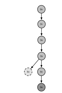
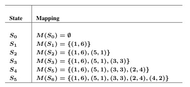
The state space tree reported in the following figures is generated by VF3 in order to verify the matching between G1 and G2 (on the left we can see a graphical representation the state space tree, while on the right the table reporting the different matching).
Starting from the void state S0, the first state explored by VF3 is S1, including the pair 1-6 (the node 1 belongs to G1 and the node 6 belongs to G2). Once verified the feasibility of this state, the new state S2 (including the pairs 1-6 and 5-1) is added and its feasibility is verified.
The algorithm proceeds until a state including all the nodes of the pattern graph will be reached (in this case S6).
We can note that after S3, the state S4, including the pairs 1-6, 5-1, 3-3, 2-4, is explored. However, it is not a feasible state according to the constraints (semantical or structural) induced by the isomorphism, thus it is discarded and the new state S5 is generated.
|

|